Sphere Scattering Effect Filter - 趣味人のブログ

This document describes details of sphere scattering effect filter. It inputs an incident wave to a rigid sphere then outputs the incident and scattered waves by the sphere. SoundObject enables a sense of leftward and rightward distance with it. Since the exact solution of the scattering by a rigid sphere is complicated, an approximate solution based on the dipole source is proposed. Next, the frequency and directional characteristics of the scattering effect by a sphere based on the proposed approximation are explained. Finally, this document describes the design and evaluation of the digital filter implementing the scattering effect by a sphere then clarifies that it enables a clearer sense of distance compared with the effects based on interaural time difference (ITD) and interaural level difference (ILD).

1. Scattering by a rigid sphere

As shown in Fig. 1, we assume a plane wave propagating to the negative direction of the x-axis as against a rigid sphere whose center is located at the origin and radius is a. Let G (jω) be a frequency transfer function representing a ratio of sound pressure observed in the surface area of the sphere to that of the plane wave. We find G (jω) from the acoustic fields of the plane wave and the scattering waves from the sphere observed at coordinate (r, θ₀). In this case, the virtual sound source position of the scattering is located at the origin. In this document, j, t, c, ω, k, and ρ denote the imaginary unit, time, acoustic speed, angular frequency of the wave, wavenumber (k = ω/c), and medium density respectively.

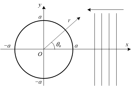
f:id:suzumushi0:20210807154509p:plain — **Fig. 1: Scattering by a rigid sphere.**

Note: The above coordinate system is different from that of SoundObject.

1.1 Exact solution

The exact solution for the above problem is well known [1]. The acoustic field of plane wave p_i is given below, where P_n denotes Legendre polynomials and j_n denotes spherical Bessel functions.

$\begin{matrix} (1) & p_{i} = \sum_{n = 0}^{\infty} j^{n} (2 n + 1) P_{n} (\cos θ_{o}) j_{n} (k r) \end{matrix}$

And the acoustic field of scattering waves p_r is given below, where h_n⁽²⁾ denotes spherical Hankel functions.

$\begin{matrix} (2) & p_{r} = - \sum_{n = 0}^{\infty} j^{n} (2 n + 1) P_{n} (\cos θ_{o}) j_{n}^{'} (k a) \frac{h_{n}^{(2)} (k r)}{h_{n}^{(2)'} (k a)} \end{matrix}$

Therefore, the frequency transfer function G (jω) representing a ratio of sound pressure observed in the surface area of the sphere to that of the plane wave is given below.

$\begin{matrix} (3) & G (j ω) = {\frac{p_{i} + p_{r}}{p_{i}}|}_{r = a} \end{matrix}$

1.2 Known approximate solutions

Since the above exact solution is computable but highly complicated, approximate solutions are proposed. [1] and [2] show approximations of scattered waves for ka ≪ 1. However, in head approximation by sphere, the frequency that gives ka = 1 is approximately 760Hz. Thus, these are unpractical for this application. Furthermore, [2] describes an approximation of scattered waves by the dipole source for kr ≪ 1, while it is also inapplicable. Therefore, this document proposes a further approximation of scattered waves by the dipole source.

1.3 Proposed approximate solution

Let Φ_i be the velocity potential of a plane wave observed at coordinate (r, θ₀). It is given below, where A is an undetermined coefficient.

$\begin{matrix} (4) & Φ_{i} = A e^{j (ω t + k x)} = A e^{j (ω t + k r \cos θ_{o})} \end{matrix}$

We approximate the scattered waves by the dipole source located at the origin. Let Φ_r be the velocity potential of scattered waves observed at coordinate (r, θ₀). It is given by the following equation, where B is also an undetermined coefficient.

$\begin{matrix} (5) & Φ_{r} = \frac{B \cos θ_{o}}{r^{2}} (1 + j k r) e^{j (ω t - k r)} \end{matrix}$

Therefore, the velocity potential Φ in the neighborhood of the sphere is given below.

$\begin{matrix} (6) & \begin{matrix} \begin{array}{r} Φ \end{array} \begin{array}{l} = Φ_{i} + Φ_{r} \\ = \{A e^{j k r \cos θ_{o}} + \frac{B \cos θ_{o}}{r^{2}} (1 + j k r) e^{- j k r}\} e^{j ω t} \end{array} \end{matrix} \end{matrix}$

To obtain the particle velocity, we find the normal derivative of the above equation.

$\begin{matrix} (7) & \begin{matrix} \begin{array}{r} \frac{\partial Φ}{\partial r} \end{array} \begin{array}{l} = [j k A \cos θ_{o} e^{j k r \cos θ_{o}} - B \cos θ_{o} \{\frac{1}{r^{3}} (2 + j k r) e^{- j k r} + \frac{j k r}{r^{3}} (1 + j k r) e^{- j k r}\}] e^{j ω t} \\ = [j k A \cos θ_{o} e^{j k r \cos θ_{o}} - \frac{B \cos θ_{o}}{r^{3}} \{{(j k r)}^{2} + j 2 k r + 2\} e^{- j k r}] e^{j ω t} \end{array} \end{matrix} \end{matrix}$

The particle velocity is 0 at r = a.

$\begin{matrix} (8) & \begin{matrix} {\frac{\partial Φ}{\partial r}|}_{r = a} = 0 \\ ∴ B = \frac{j k a^{3} A e^{j k a \cos θ_{o}}}{\{{(j k a)}^{2} + j 2 k a + 2\} e^{- j k a}} \end{matrix} \end{matrix}$

Thus, the velocity potential Φ in the neighborhood of the sphere is given below.

$\begin{matrix} (9) & Φ = \{A e^{j k r \cos θ_{o}} + \frac{j k a^{3} A e^{j k a \cos θ_{o}}}{\{{(j k a)}^{2} + j 2 k a + 2\} e^{- j k a}} \frac{\cos θ_{o}}{r^{2}} (1 + j k r) e^{- j k r}\} e^{j ω t} \end{matrix}$

Finally, the velocity potential in the surface area of the sphere is given below.

$\begin{matrix} (10) & {Φ|}_{r = a} = A e^{j (ω t + k a \cos θ_{o})} \{1 + \frac{j k a (1 + j k a) \cos θ_{o}}{{(j k a)}^{2} + j 2 k a + 2}\} \end{matrix}$

2. Transfer function of scattering effect by sphere

Based on the above discussions, the frequency transfer function G (jω) representing a ratio of sound pressure observed in the surface area of the sphere to that of the plane wave is given below.

$\begin{matrix} (11) & \begin{matrix} \begin{array}{r} G (j ω) \end{array} \begin{array}{l} = {\frac{ρ \frac{\partial Φ}{\partial t}}{ρ \frac{\partial Φ_{i}}{\partial t}}|}_{r = a} = {\frac{j ω Φ}{{j ω Φ}_{i}}|}_{r = a} \\ = 1 + \frac{j k a (1 + j k a) \cos θ_{o}}{{(j k a)}^{2} + j 2 k a + 2} \\ = 1 + \frac{{(j a ω)}^{2} + j a c ω}{{(j a ω)}^{2} + j 2 a c ω + 2 c^{2}} \cos θ_{o} \end{array} \end{matrix} \end{matrix}$

The transfer function G (s) corresponding to the above frequency transfer function G (jω) is given below, where ω_c = c /a.

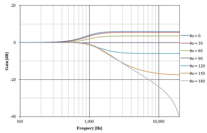
$\begin{matrix} (12) & \begin{matrix} \begin{array}{r} G (s) \end{array} \begin{array}{l} = 1 + \frac{a^{2} s^{2} + a c s}{a^{2} s^{2} + 2 a c s + 2 c^{2}} \cos θ_{o} \\ = 1 + \cos θ_{o} - \frac{ω_{c} (s + 2 ω_{c}) \cos θ_{o}}{s^{2} + 2 ω_{c} s + 2 {ω_{c}}^{2}} \end{array} \end{matrix} \end{matrix}$

An example of frequency characteristics of G (jω) is shown below, where c = 343.7 m/s and a = 71.5 mm.

f:id:suzumushi0:20210807160042p:plain — **Fig. 2: An example of frequency characteristics of scattering effect by a sphere.**

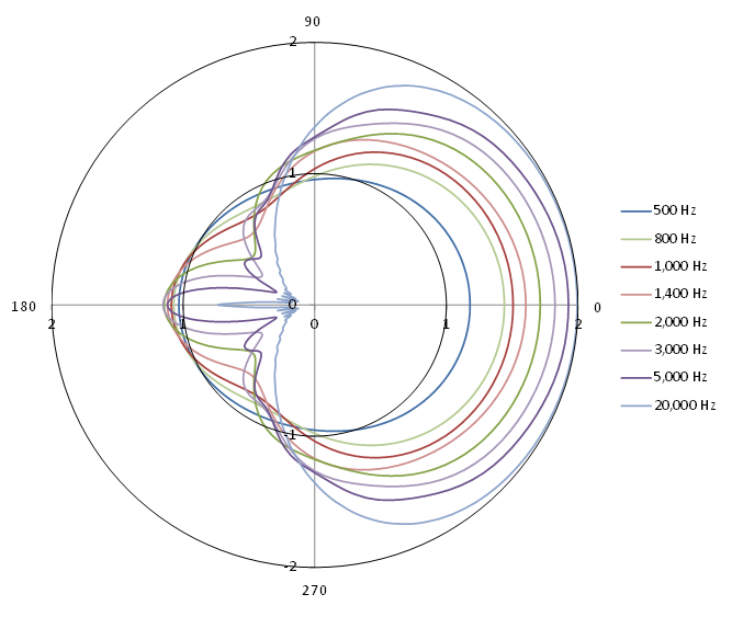
And an example of directional characteristics of G (jω) is also shown below, where the radius direction and angle from the x-axis show gain (ratio) and θ_o respectively. The frequency whose wave length is equal to the diameter of the sphere is approximately 2,400Hz. The figure illustrates that the incident wave less than 2,000Hz is significantly propagated to the behind of the sphere. However, over 2,000Hz, differences in the front directional gain are rarely observed. Furthermore, over 3,000Hz, there is no significant difference in the directional characteristics.

f:id:suzumushi0:20211027192258p:plain — **Fig. 3: An example of directional characteristics of scattering effect by a sphere.**

For reference, an example of directional characteristics of the frequency transfer function based on the exact solution numerically calculated from equation (3) is shown below. Although slight differences are observed in detail, directional characteristics tendencies based on the exact and approximate solutions are the same. Since head is not a strictly rigid sphere, sufficient effects are expected by the proposed approximate solution.

f:id:suzumushi0:20211027192326p:plain — **Fig. 4: An example of directional characteristics based on the exact solution.**

Note: A numerical calculation program of the exact solution is available on the following link.

github.com

3. Sphere scattering effect filter

With bilinear transformation, we find an infinite impulse response (IIR) filter that implements a system transfer function H (z) equivalent to the transfer function G (s) denoted by equation (12). Bilinear transform-based design method for IIR filters is well-known, thus leaving out a detailed explanation. If needed, refer to the following document. (In Japanese).

suzumushi0.hatenablog.com

The correspondence relationship between angular frequencies of the transfer function G (s) and system transfer function H (z) is warped by bilinear transformation. Therefore, compensated angular frequency ω_a corresponding to ω_c is shown below, where T denotes sampling interval.

$\begin{matrix} (13) & ω_{a} = \tan (\frac{ω_{c} T}{2}) = \tan (\frac{c T}{2 a}) \end{matrix}$

Thus, the system transfer function H (z) is given below.

$\begin{matrix} (14) & \begin{array}{l} H (z) = {G (s)|}_{s = \frac{1 - z^{- 1}}{1 + z^{- 1}}, ω_{c} = ω_{a}} \\ = 1 + \cos θ_{o} - \frac{ω_{a} (\frac{1 - z^{- 1}}{1 + z^{- 1}} + 2 ω_{a}) \cos θ_{o}}{{(\frac{1 - z^{- 1}}{1 + z^{- 1}})}^{2} + 2 ω_{a} \frac{1 - z^{- 1}}{1 + z^{- 1}} + 2 {ω_{a}}^{2}} \\ = 1 + \cos θ_{o} - \frac{ω_{a} \{(2 ω_{a} + 1) + 4 ω_{a} z^{- 1} + (2 ω_{a} - 1) z^{- 2}\} \cos θ_{o}}{(2 {ω_{a}}^{2} + 2 ω_{a} + 1) + 2 (2 {ω_{a}}^{2} - 1) z^{- 1} + (2 {ω_{a}}^{2} - 2 ω_{a} + 1) z^{- 2}} \\ = 1 + \frac{\{(ω_{a} + 1) - 2 z^{- 1} - (ω_{a} - 1) z^{- 2}\} \cos θ_{o}}{(2 {ω_{a}}^{2} + 2 ω_{a} + 1) + 2 (2 {ω_{a}}^{2} - 1) z^{- 1} + (2 {ω_{a}}^{2} - 2 ω_{a} + 1) z^{- 2}} \end{array} \end{matrix}$

The above could be essentially implemented as a second-order IIR filter (biquad filter). An example of frequency characteristics of the above digital filter is shown below, where T = 1 /44,100 s.

f:id:suzumushi0:20210807161050p:plain — **Fig. 5: An example of frequency characteristics of sphere scattering effect filter.**

4. Evaluation

SoundObject could select the output from scattered waves by the sphere and incident wave with ITD and ILD. Therefore, the sphere scattering effect filter could be evaluated with comparisons of these outputs. As shown in the following video, the latter output sounds like the acoustic source locates close to the ear regardless of the distance. On the other hand, the former demonstrates a clearer sense of distance enabled by the sphere scattering effect filter.

www.youtube.com

References

[1] P. M. Morse, "Vibration and Sound, Second Ed.," International series in pure and applied physics, McGRAW-HILL, 1948.
[2] T. Ito, "Principles of Acoustic Engineering," Corona Publishing, 1955 (In Japanese). Acoustic Lab. - Waseda Univ.